Once absorbed by a GHG molecule, the GhIR energy will be re-radiated and absorbed very many times before it will be radiated out into space or be absorbed by the surface.
Describing this process quantitatively in formulas seemed to be impossible, at least for my mathematics skills. And as far as I know, even very skilled mathematicians have never been able to describe more than 7 layers in a mathematical model of the atmosphere. So I invented another way to calculate a large number of layers accurately, using an iteration approach.
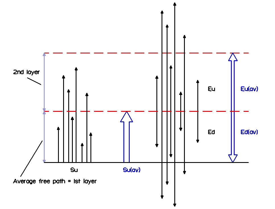
Let me first show the layer definition image of the first chapter:
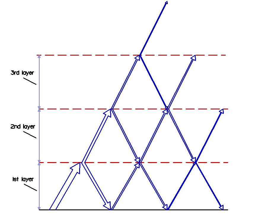
If I tilt the blue arrows a bit, a new image appears, that can clarify the formulas that I based my simulation on:
You see that Su is divided equally in Ed1 and Eu1.
Ed1 looses 50% to the surface, and Eu1 looses 50% to layer 3, so half of Ed1 and Eu1 (twice 25% of Su) will be re-radiated back to the top of layer 1.
In the next iteration we see that the amount of energy coming from the top of layer 2 is more than that coming from the surface. This shows how the atmosphere is “drained” by the absorption at the surface, as was already mentioned in chapter 1.
The simulation
I tried to simulate this process in a spreadsheet, at first for just a 6 layers atmosphere.
Once I found the right way to do that, the rest of the spreadsheet was very simple.
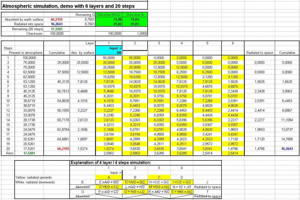
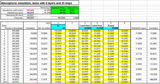
Below you see a demo that shows the way the Su (surface upward ) radiation would behave in an atmosphere with 6 layers, followed over 20 iterations (click twice for enlargement).
This time the energy flows from left to right:
Calculating the re-radiation of Su
The left side of layer 1 is the surface of the earth, the right side of layer 6 is space.
At the top of the right side of layer 1 I added 100 W/m2 as the GhIR part of the Su (surface upward) radiation that is absorbed. I chose 100 W/m2 in order to make the energy “read” like a percentage.
In the explanation window with the 4 layer/ 4steps model under the demo, you see with which formula this energy is iteratively reradiated upwards (yellow) and downwards (white).
In the thin diagonal lines you recognise the blue arrows of the iteration scheme.
In the demo you see that 25% is immediately absorbed by the surface in the first step, leaving only 75% of the energy in the atmosphere.
Since it is a 6 layer model, it takes 6 iterations (steps) to also start loosing energy into space (right side) . By then over 45% of the energy is already lost to the earth surface.
After 20 iterations still 17,5% is left in the atmosphere, so it is clear that many more iterations are necessary for a really accurate outcome, even in a simulation with so few layers.
As you can see, I always take the remaining energy (the energy that is still in the atmosphere after the last iteration), divide it by two and add it to the Ed and Eu.
Even after a lot of iterations, especially in multi layered simulations, the remaining energy can still be considerable, but since it is very evenly distributed, this 50% division is quite accurate.
A helpful image may be this one of a 7 layer (multi iterative) demo.
The column width suggests how the layers get thicker with height:
Adding other energy sources
The brilliant thing of this spreadsheet is that it is extremely easy to replace immensely complex math. What about adding the sunlight’s IR that is absorbed when entering the atmosphere?
Simply add it to the layer(s) in which it is absorbed. Let’s say that is layer 5. Then I can just type in the amount and right away this energy is distributed and calculated.
So let’s use realistic figures: Su (without the IR window part) of 300 W/m2 and absorbed sunlight IR of 70 W/m2.
Just for fun we also add latent heat that is released by condensation in layers 3 and 4 as 2x 60 W/m2
Takes 3 seconds and voila, the ratio becomes 61.7% vs 38.3%:
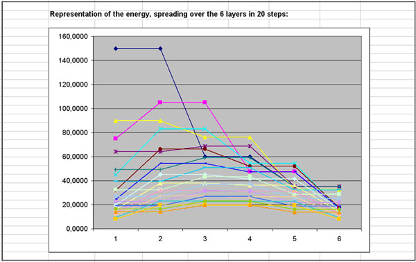
It is also possible to represent a simulation run in a graph.
Here you see how the Su energy is spreading over the atmosphere in 20 steps.
After the last step (orange) it is quite symmetrically distributed already:
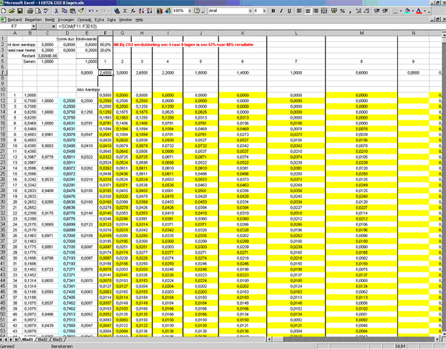
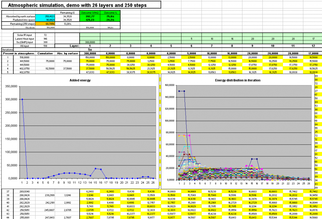
By the magic of Excel this demo model is extendable in only a few minutes to a full scale atmospheric model of 26 layers and 250 iterations.
I added latent heat and absorbed solar IR rather intuitively, which has big consequences, as will be discussed later.
I show the left top part (click to enlarge):
The right graph shows the redistribution of energy during the iteration (the first 200 steps).
The left one shows my input of energy by Su, Solar IR and latent heat (LH), in the respective layers.
Try your own simulation
Of course you want to play with this funny tool yourself. Well, here it is.
The only variable in the simulation is the energy input, the rest are basic formula’s.
So feel free to change it, by changing the numbers in the pale green section.
My choices:
– Su, the amount of IR that is radiated upwards from the surface (the IR window excluded), by definition is absorbed at the top of layer 1.
– Latent heat is transported upwards in water vapour untill it condenses. Then it changes into real energy, warming the atmosphere. I chose a lot of layers to do that.
– Solar IR is absorbed in two parts: the part that is CO2 sensitive in the highest layers, the part that is H2O sensitive much lower. My choice of layers was rather intuitive.
Have fun!
Some minor changes were made to the text of this chapter.