1. The Fireworks Theory for greenhouse gases

IR radiation behaviour
I started with imagining how IR radiation would behave when radiated from the earth’s surface.
Of course some wavelengths will radiate directly into space through the IR window.
All the rest would at a certain point be absorbed by a greenhouse gas (GHG) molecule.
Once absorbed, in an equilibrium situation, the same amount of energy would be re-radiated
evenly in all directions by the molecule.

Note: in the equilibrium situation, the frequency of the absorbed IR energy is “lost”, since
we assume all GHG molecules in a certain volume to have the same temperature, and they all
will radiate out energy in their own spectrum. So the spectrum of the re-radiation is only
related to the concentration of the different GHG at that particular place, not related to the
absorbed wavelength.

Since we are only interested in the vertical energy transport by radiation, we assume that only
the vertical component of all that radiation is effective, so effectively 50% of the energy radiated
from that molecule ends up going upwards, and 50% going downwards.

Note: since the earth is a sphere, some radiation that is downwards but very close to
horizontal, will still escape into space. This effect should be calculated to increase the accuracy
of the model.

This radiation in its turn will be absorbed by other GHG molecules, which in their turn will reradiate
into all directions. The graphic representation of that mechanism looks like fireworks, thus providing a
suitable name for my theory.

 

 

So far nothing new, this is basic radiation theory.

The next step is trying to quantify this principle.
Many have tried that before, by describing the atmosphere in multi layer models and calculating
the energy exchange, using temperature, pressure, mass, warmth capacity and heavy mathematics.

Free path based layers
Although my set-up looks a lot like the multilayered models, it is fundamentally different, by the way
I define my layers.
Here’s the trick:

The top side of my first layer is defined as the distance above the surface, equal to
the average vertical free path of the GHG sensitive IR radiation (GhIR).

In other words, the top of my first layer, is by definition the height at which in average the greenhouse gas sensitive IR radiation has been absorbed. Because the GHG concentration is rather equally distributed, I assume that approximately half of the GhIR will actually have been absorbed at this height.

The thickness of the next layer is again defined by the next average free path of GhIR.

In a homogenous atmosphere all layers would have the same thickness, but because of the
dramatic decrease of H2O vapour with height due to condensation, and the lower pressure coming with height, the layers get thicker fast.

Follow the photon
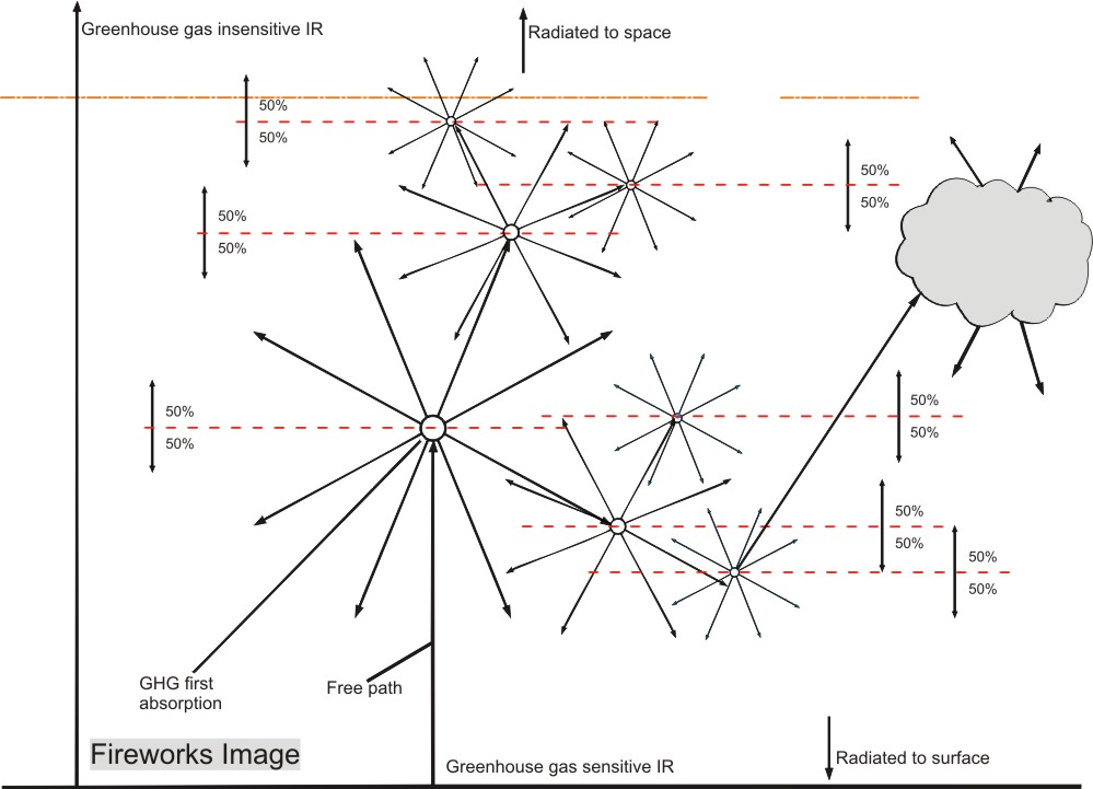
Let’s have a closer look at this fireworks process. An image may help to understand the definition:

First we look at the greenhouse sensitive radiation that comes from the earth:  Surface upward (Su).
Because of different sensitivities for GH gases for different wavelengths, but also because of statistics (hitting a GHG molecule is a matter of probability for a photon) the Su is absorbed over a wide height range. But we can define a layer which is bordered by the average height at which the Su is absorbed, the blue arrow Su(av).

The absorbed energy will be re-radiated as in the fireworks impression image, but for our model, we assume it is all radiated from the top of the layer, resulting in equal energy flows of 50% up (Eu) and 50% down (Ed).
Ed will reach the surface after having been 50% absorbed, because the surface is at average absorption distance.
Eu will by definition in average be absorbed at the top of the second layer. Due to the thinner air and the lower water vapour content, this layer will be thicker.

This process can be repeated until all energy is either radiated to space, or absorbed by the surface.
So, if the amount of layers is known, the resulting distribution ratio (Ed/Eu) can be calculated too.

Why this weird definition of layers?
The great advantages of this approach will become clear later on, when implemented in my
atmospheric simulation model. As a clarification I first would like to refer to an analogue way of
thinking, used in road mapping.

The Fireworks theory analogy of roadmapping
When you are mapping an area, you will choose to define the roads by their length. That way
travellers can choose the shortest way to their destination
People also know how fast their car drives so the distance tells them at what time they will most
likely arrive at their destination .
But in crowded area’s they should calculate the delay by traffic jams and traffic lights in order to be
able to make an accurate estimation. That takes a lot of data. At what time will I drive? Howe many
traffic jams are expected on that particular day? And comparing all possible routes to establish the
fastest one is close to impossible.

In fact, in an urban area the exact physical representation on normal maps in km does not give any
useful  information to the traveller.

That is why a map with not distance but driving time as the graphical representation, is far more
useful. It is easy to make by statistical analysis over the last few years of a particular day and time,
and would easily show the traveller in one glimps of an eye which road is the fastest way to reach
his destination. The trick is that all variables (traffic jams, detours, but also distance) are integrated in the parameter “traveling time”.

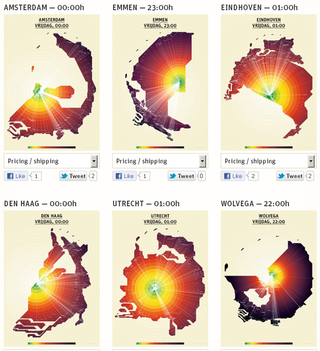
Looking for examples on internet I found a site that does something similar: show the Dutch map as a
function of travelling time by public transport. This is the actual real time app, which is quite fun to play with (use the scrolling wheel and the bar of “afgelopen 24 U”).

First I show a normal map of the Netherlands:

Than a representation of the Netherlands in travelling time by public transport from a certain city at a
certain time:

Of course the problems are just shifted to the making of the maps, but that obviously is far more efficient than to have every traveller calculate his route every time.
In this case, the maps can be produced almost real-time by a computer that has access to the public transport database, and are far more useful than a normal map.

In the same way as in the analogy, I define my layers as the free path of a GhIR photon, and shift all problems to the establishing of the free path length.

Temperature and pressure
Now, here is where you will have to stretch your braincells to the max!

The main advantage of my layer definition is that this set-up completely eliminates temperature and pressure out of the calculations.

For climate experts this must be very hard to accept.
But it really works that way. Just the same way as the kilometers are out of the travelling time map: by definition.
Together with the sensitivity spectrum of IR for GHG, temperature and pressure determine the free path of the GhIR, so they are already fully integrated in the model, once we have determined the number of layers.

I will explain in chapter 2 what this layer definition results into when it is used in a simulation.

How are pressure and temperature embedded in layer thickness?
The logic of the Fireworks image is quite convincing: since no energy can get lost, it is possible to follow all absorbed energy by just following the 50% rule and see where it ends up: at the surface or in space.
But how can pressure and temperature be left out of the calculation?

Pressure of course translates into the density of GHG molecules, and thus into the layer thickness. It is easy to understand that it is well represented in the layer thickness and the number of layers.

Temperature is a lot harder to understand.
If we only consider radiation, the absorbed energy is by definition equal to the energy that is radiated out, because we are talking about an equilibrium situation. If the GHG molecule receives more or less energy than it radiates out, it’s temperature will change until absorption and radiation are equal again. Temperature is a result, not a given value.  Whatever temperature it has: the molecule will radiate it’s absorbed energy up 50% and down 50%.

Convection and latent heat
If we also consider convection and latent heat transport, the resulting temperature of the greenhouse gas molecules will be determined by the total amount of acquired energy by both radiation and the other influences.

The temperature of the atmosphere below the tropopause, under which there is a lot of convection, seems to be determined by the wet or dry adiabatic lapse rate, as is explained in chapter 10.
But that is not exactly the case! Because of the radiation transfer process, powered by the fireworks principle, the proces of convection is not entirely adiabatic, and radiation energy will slightly change the temperature of the air during convection.

The other way around, also the radiation process is influenced by convection, changing the warming properties of an increased GHG concentration substantially, as is explained in chapter 8.

For a realistic radiation model of the atmosphere, the other radiation variables like incoming IR from the sun, and LWIR radiation emerging from latent heat energy from condensation of water vapour in te mid and lower atmosphere, have to be taken into account. But as you will see in the next chapter, that can be done surprisingly easy with the fireworks simulation.